Note: Descriptions are shown in the official language in which they were submitted.
CA 02997013 2018-02-28
DESCRIPTION
ISING MODEL QUANTUM COMPUTATION DEVICE
Technical Field
[0001]
The present disclosure shows a quantum computation device
capable of easily solving the Ising model to easily solve an
NP-complete problem or the like mapped into the Ising model.
Background Art
[0002]
The Ising model has been researched originally as a model
of a magnetic material but recently it is paid attention as a
model mapped from an NP-complete problem or the like. However,
it is very difficult to solve the Ising model when the number
of sites is large. Thus, a quantum annealing machine and a
quantum adiabatic machine in which the Ising model is implemented
are proposed.
[0003]
In the quantum annealing machine, after Ising interaction
and Zeeman energy are physically implemented, the system is
sufficiently cooled so as to realize a ground state, and the
ground state is observed, whereby the Ising model is solved.
However, in a case where the number of sites is large, the system
is trapped into a metastable state in the process of being cooled,
and the number of the metastable state exponentially increases
with respect to the number of sites, whereby there is a problem
1
CA 02997013 2018-02-28
in that the system is not easily relaxed from the metastable
state to the ground state.
[0004]
In the quantum adiabatic machine, transverse magnetic
field Zeeman energy is physically implemented, and then the
system is sufficiently cooled to realize the ground state of
only the transverse magnetic field Zeeman energy. Then, the
transverse magnetic field Zeeman energy is gradually lowered,
Ising interaction is physically implemented slowly, the ground
state of the system that includes the Ising interaction and
vertical magnetic field Zeeman energy is realized, and ground
state is observed, whereby the Ising model is solved. However,
when the number of sites is large, there is a problem in that
the speed of gradually lowering the transverse magnetic field
Zeeman energy and physically implementing the Ising interaction
needs to be exponentially decreased with respect to the number
of sites.
[0005]
In a case where the NP-complete problem or the like is
mapped into an Ising model, and the Ising model is implemented
as a physical spin system, there is a problem of a natural law
that Ising interaction between sites that are physically located
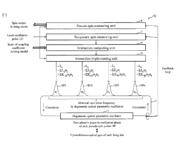
close to each other is high, and Ising interaction between sites
that are physically located far from each other is low. The
reason for this is that, in an artificial Ising model in which
the NP-complete problem is mapped, there may be cases where Ising
interaction between sites that are physically located close to
2
CA 02997013 2018-02-28
each other is low, and Ising interaction between sites that are
physically located far from each other is high. The difficulty
in mapping into a natural spin system also makes it difficult
to easily solve the NP-complete problem or the like.
Citation List
Patent Literature
[0006]
Patent Literature 1: Japanese Patent No. 5354233
Patent Literature 2: Japanese Patent Laid-open No.
2014-134710
Non-Patent Literature
[0007]
Non-Patent Literature 1: Z.Wang,A.Marandi, K. Wen, R.L.
Byer and Y. Yamamoto, "A Coherent Ising Machine Based on
Degenerate Optical Parametric Oscillators," Phys. Rev. A88,
063853 (2013).
Summary of the Invention
Technical Problem
[0008]
Patent Literatures 1 and 2 and Non-Patent Literature 1
for solving the above problems are described. An NP-complete
problem can be substituted by an Ising model of a magnetic
material, and the Ising model of the magnetic material can be
substituted by a network of a laser or laser pulse.
[0009]
3
CA 02997013 2018-02-28,
Here, in the Ising model of a magnetic material, in a pair
of atoms interacting with each other, the directions of spins
tend to be oriented in opposite directions (in the case of
interaction of antiferromagnetism) or in the identical direction
(in the case of interaction of ferromagnetism) such that the
energy of spin alignment is the lowest.
[0010]
On the other hand, in a network of lasers or laser pulses,
in a pair of lasers or laser pulses interacting with each other,
the polarizations or phases of oscillation tend to be reverse
rotations or opposite phases (in the case of interaction of
antiferromagnetism) , or the identical rotation or the identical
phase (in the case of interaction of ferromagnetism)
respectively such that the threshold gain of the oscillation
mode is the lowest.
[0011]
In other words, in the system configured by one pair of
lasers or laser pulses, the polarization or phases of oscillation
can be optimized such that the threshold gain of the oscillation
mode is the lowest. On the other hand, in the system configured
by many pairs of lasers or laser pulses, when an attempt to
optimize the polarizations or phases of oscillation is made for
a "certain" pair of lasers or laser pulses, the polarization
or phases of oscillation cannot be optimized for "the other"
pairs of lasers or laser pulses. Therefore, in the system
configured by many pairs of lasers or laser pulses, a "point
of compromise" on the polarizations or phases of oscillation
4
CA 02997013 2018-02-28
as the "overall" network of lasers or laser pulses is searched
for.
[0012]
However, in a case where the polarization or phases of
oscillation are optimized in the overall network of lasers or
laser pulses, it is necessary to make an attempt to achieve
synchronization between the lasers or laser pulses so as to
establish a single oscillation mode in the overall network of
lasers or laser pulses instead of establishing individual
oscillation modes in the respective pairs of lasers or laser
pulses.
[0013]
As described above, according to Patent Literatures land
2 and Non-Patent Literature 1, the pumping energy of each laser
or laser pulse is controlled, a single oscillation mode which
minimizes the threshold gain in the overall network of lasers
or laser pulses is established, the polarization or phase of
oscillation of each laser or laser pulse is measured, and the
direction of each Ising spin is finally measured. Therefore,
the problems of the trapping into the metastable states and the
implementation rate of the Ising interaction in the quantum
annealing machine and the quantum adiabatic machine can be
solved.
[0014]
In addition, according to Patent Literatures 1 and 2 and
Non-Patent Literature 1, it is possible to freely control not
only the magnitude of Ising interaction between sites physically
CA 02997013 2018-02-28
located close to each other but also the magnitude of Ising
interaction between sites physically located far from each other.
Accordingly, the artificial Ising model mapped from an
NP-complete problem or the like can be solved regardless of the
physical distances between the sites.
[0015]
Next, Patent Literatures 1 and 2 are concretely explained.
First, the magnitude and sign of the pseudo Ising interaction
between two surface emission lasers are implemented by
controlling the amplitudes and phases of light exchanged between
the two surface emission lasers. Next, the pseudo Ising spins
of the respective surface emission lasers are measured by
measuring the polarization or phases of oscillation in the
respective surface emission lasers after the respective surface
emission lasers reach a steady state during the light exchange
process.
[0016]
At this time, in order to establish a single oscillation
mode in which the polarizations or phases of oscillation in the
overall network of surface emission lasers are optimized, it
is necessary to achieve synchronization between the surface
emission lasers. Therefore, the oscillation frequencies of the
surface emission lasers are equalized to an identical frequency
by using injection locking from a master laser to the surface
emission lasers. However, because the free-running frequencies
of the surface emission lasers are slightly different from the
oscillation frequency of the master laser, the phases of
6
CA 02997013 2018-02-28
oscillation of the surface emission lasers in the initial state
are unbalanced toward the zero phase or n phase in the oscillation
of the surface emission lasers in the steady states.
Resultantly, incorrect answers are likely to be caused by the
unbalanced phases in the initial states.
[0017]
In addition, in the case where the number of Ising sites
is M, the surface emission lasers in the number M are needed,
and M(M-1)/2 optical paths are needed between the surface
emission lasers. Further, the magnitude and sign of the pseudo
Ising interaction between the surface emission lasers cannot
be precisely implemented unless the lengths of the optical paths
between the surface emission lasers are precisely adjusted.
Therefore, in the case where the number of the Ising sites is
large, the Ising model quantum computation device becomes
massive and complex.
[0018]
Next, Non-Patent Literature 1 is explained concretely.
First, the magnitude and sign of the pseudo Ising interaction
between two laser pulses are implemented by controlling the
amplitudes and phases of light exchanged between the two laser
pulses. Next, the pseudo Ising spins of the respective laser
pulses are measured by measuring the phases of oscillation in
the respective laser pulses after the respective laser pulses
reach a steady state during the light exchange process.
7
CA 02997013 2018-02-28
[0019]
At this time, in order to establish a single oscillation
mode in which the phases of oscillation in the overall network
of laser pulses are optimized, it is necessary to achieve
synchronization between the laser pulses. Therefore, the
oscillation frequencies of the laser pulses are equalized to
an identical frequency by using a degenerate optical parametric
oscillator and a ring resonator. In addition, because the
down-conversion by the degenerate optical parametric oscillator,
instead of the injection locking by the master laser, is used,
the phases of oscillation of the laser pulses in the initial
state are not unbalanced toward the zero phase or n phase in
the oscillation of the laser pulses in the steady states.
Resultantly, the incorrect answers caused by the unbalanced
phases in the initial states are unlikely to occur.
[0020]
Then, a first method to realize a technique disclosed in
Non-Patent Literature 1 is explained concretely. According to
the first method, a modulator which controls the amplitudes and
phases of the light exchanged between laser pulses is arranged
on a delay line which has a length equal to the interval of the
laser pulses, branches from the ring resonator, and joins the
ring resonator. Part of preceding laser pulses propagate
through the delay line and are modulated by the modulator, and
subsequent laser pulses propagate in the ring resonator and do
not propagate through the delay line, so that these laser pulses
are combined, and resultantly light is exchanged between the
8
CA 02997013 2018-02-28,
laser pulses. While the circular propagation of the laser
pulses in the ring resonator in the above manner is repeated,
the phases of the laser pulses are measured after the laser pulses
reach a steady state.
[0021]
Thus, in the case where the number of the Ising sites is
M, (M-1) types of delay lines are needed, and the (M-1) modulators
are needed. In addition, unless the lengths of the delay lines
(equal to the interval between the laser pulses) are precisely
adjusted, the magnitude and sign of the pseudo Ising interaction
between the laser pulses cannot be precisely implemented.
Therefore, in the case where the number of the Ising sites becomes
large, the Ising model quantum computation device becomes
massive and complex even according to the first method.
[0022]
Next, a second method for realizing the technique
disclosed in Non-Patent Literature 1 is explained concretely.
According to the second method, a detector which measures the
phases of the laser pulses is arranged at the branching position
from the ring resonator. In addition, a computer which computes
interactions in the Ising model on the basis of coupling
coefficients in the Ising model and the measured phases of the
laser pulses is arranged. Further, a modulator which controls
the amplitudes and phases of light injected to the laser pulses,
on the basis of the computed interactions in the Ising model,
is arranged at the joining position to the ring resonator. While
the feedback loop constituted by the detector, the computer,
9
CA 02997013 2018-02-28
and the modulator as above is repeated, the phases of the laser
pulses are measured after the laser pulses reach a steady state.
[0023]
Thus, even in the case where the number of Ising sites
is M, the necessary number of each of the detector, computer,
and modulator is only one. In addition, neither the optical
paths (in Patent Literatures 1 and 2) nor the delay lines
(according to the first method) , the lengths of which should
be precisely adjusted, are necessary. Therefore, even in the
case where the number of the Ising sites becomes large, the Ising
model quantum computation device becomes small and simple.
[0024]
Further, it is desirable that the pseudo Ising
interaction between laser pulses be close to an instant
interaction and not be a delay interaction. Therefore, it is
desirable that the computer compute all interactions in the Ising
model relating to all the laser pulses after the detector
measures the phases of all the laser pulses before all the laser
pulses "circulate once" in the ring resonator and the modulator
controls the amplitudes and phases of light injected to all the
laser pulses.
[0025]
However, since the time for the computer computing all
interactions in the Ising model relating to all the laser pulses
increases in proportion to the square of the number of the Ising
sites (in the case of the two-body Ising interactions) , it can
be considered that when the number of Ising sites becomes large
,
the above computing time becomes longer than the time in which
all the laser pulses "circulate once" in the ring resonator, due
to limitations of clock signals and memories in the computer.
[0026]
In order to solve the above problems, the object of the
present disclosure is to secure sufficient time for computing
all interactions in the Ising model relating to all the laser
pulses during the process in which the feedback loop constituted
by the Ising spin measuring step, the Ising interaction computing
step, and the Ising interaction implementing step is repeated,
and thereby stabilize the operations in the entire system and
lower the possibility of occurrence of incorrect answers even
in the case where the number of the Ising sites is large.
Solution to Problem
[0027]
In one aspect of the invention, there is provided an Ising
model quantum computation device comprising: a degenerate
optical parametric oscillator which causes degenerate optical
parametric oscillation of a plurality of pseudo spin pulses
corresponding to a plurality of spins in the Ising model and
having an identical oscillation frequency; a ring resonator
which circularly propagates the plurality of pseudo spin pulses;
a temporary spin measuring unit which temporarily measures
pseudo spins of the plurality of pseudo spin pulses by
temporarily measuring phases of the plurality of pseudo spin
pulses every time the plurality of pseudo spin pulses circularly
propagate in the ring resonator, and suspends measurement after
11
CA 2997013 2019-04-24
one set of measurement is completed before another set of
measurement is restarted; an interaction computing unit which
temporarily computes all interactions relating to the plurality
of pseudo spin pulses, on the basis of the coupling coefficients
of the Ising model and the pseudo spins of the plurality of pseudo
spin pulses which the temporary spin measuring unit has most
recently measured, after the temporary spin measuring unit
completes one set of measurement before the temporary spin
measuring unit restarts another set of measurement; an
interaction implementing unit which temporarily implements
magnitudes and signs of all the interactions relating to the
plurality of pseudo spin pulses which the interaction computing
unit has most recently computed, by controlling amplitudes and
phases of light injected to the plurality of pseudo spin pulses,
after the interaction computing unit completes a temporary
computation of all the interactions relating to the plurality
of pseudo spin pulses; and a pseudo spin measuring unit which
measures the pseudo spins of the plurality of pseudo spin pulses
by measuring the phases of the plurality of pseudo spin pulses
after the plurality of pseudo spin pulses reach a steady state
while a feedback loop constituted by steps performed by the
temporary spin measuring unit, the interaction computing unit,
and the interaction implementing unit is repeated.
[0027a]
In order to achieve the above object, the time in which
all the laser pulses "circulate once" in the ring resonator is
effectively lengthened. In the Ising spin measuring step, the
ha
CA 2997013 2019-04-24
measurement is suspended after one set of measurement of all
Ising spins is completed before another set of measurement of
all the Ising spins is restarted. In the Ising interaction
computing step, all Ising interactions relating to all the Ising
spins can be computed with a sufficient time margin on the basis
of the measurement of the Ising spins which has been most recently
performed, after one set of measurement of all Ising spins is
llb
CA 2997013 2019-04-24
completed before another set of measurement of all the Ising
spins is restarted by the Ising spin measuring step.
[0028]
Specifically, the present disclosure is an Ising model
quantum computation device, characterized in including: a
degenerate optical parametric oscillator which causes
degenerate optical parametric oscillation of a plurality of
pseudo spin pulses corresponding to a plurality of spins in the
Ising model and having an identical oscillation frequency; a
ring resonator which circularly propagates the plurality of
pseudo spin pulses; a temporary spin measuring unit which
temporarily measures pseudo spins of the plurality of pseudo
spin pulses by temporarily measuring phases of the plurality
of pseudo spin pulses every time the plurality of pseudo spin
pulses circularly propagate in the ring resonator, and suspends
measurement after one set of measurement is completed before
another set of measurement is restarted; an interaction
computing unit which temporarily computes all interactions
relating to the plurality of pseudo spin pulses, on the basis
of coupling coefficients of the Ising model and the pseudo spins
of the plurality of pseudo spin pulses which the temporary spin
measuring unit has most recently measured, after the temporary
spin measuring unit completes one set of measurement before the
temporary spin measuring unit restarts another set of
measurement; an interaction implementing unit which temporarily
implements magnitudes and signs of all the interactions relating
to the plurality of pseudo spin pulses which the interaction
12
CA 2997013 2019-04-24
computing unit has most recently computed, by controlling
amplitudes and phases of light injected to the plurality of
pseudo spin pulses, after the interaction computing unit
completes a temporary computation of all the interactions
relating to the plurality of pseudo spin pulses; and a pseudo
spin measuring unit which measures the pseudo spins of the
plurality of pseudo spin pulses by measuring the phases of the
plurality of pseudo spin pulses after the plurality of pseudo
spin pulses reach a steady state while a feedback loop
constituted by steps performed by the temporary spin measuring
unit, the interaction computing unit, and the interaction
implementing unit.
[0029]
According to the above structure, the time in which all
the laser pulses "circulate once" in the ring resonator is
effectively lengthened. Therefore, in the Ising interaction
computing step, all Ising interactions relating to all the Ising
spins can be computed with a sufficient time margin on the basis
of the measurement of the Ising spins which has been most recently
performed.
[0030]
In addition, the present disclosure is an Ising model
quantum computation device, characterized in that the ring
resonator circularly propagates the plurality of successive
pseudo spin pulses, which correspond to the plurality of spins
in the Ising model; and the plurality of pseudo spin pulses
circularly propagating in the ring resonator each pass once or
13
CA 2997013 2019-04-24
=
more times the position of the branch from the ring resonator
to the temporary spin measuring unit, after the temporary spin
measuring unit completes one set of measurement before the
temporary spin measuring unit restarts another set of
measurement.
[0031]
According to the above structure, in the Ising
interaction computing step, all the Ising interactions relating
to all the Ising spins can be computed with a sufficient time
margin on the basis of the measurement of the Ising spins which
has been most recently performed, while the plurality of pseudo
spin pulses each pass once or more times the position of the
branch from the ring resonator to the temporary spin measuring
unit.
[0032]
In addition, the present disclosure is an Ising model
quantum computation device, characterized in that the ring
resonator circularly propagates the plurality of successive
pseudo spin pulses corresponding to the plurality of spins in
the Ising model, and a plurality of successive dummy pulses which
do not correspond to the plurality of spins in the Ising model;
and the plurality of dummy pulses circularly propagating in the
ring resonator each pass once the position of a branch from the
ring resonator to the temporary spin measuring unit, after the
temporary spin measuring unit completes one set of measurement
before the temporary spin measuring unit restarts another set
of measurement.
14
CA 2997013 2019-04-24
CA 02997013 2018-02-28
[0033]
According to the above structure, in the Ising
interaction computing step, all the Ising interactions relating
to all the Ising spins can be computed with a sufficient time
margin on the basis of the measurement of the Ising spins which
has been most recently performed, while the plurality of dummy
pulses each pass once the position of the branch from the ring
resonator to the temporary spin measuring unit.
[0034]
In addition, the present disclosure is an Ising model
quantum computation device, characterized in that the degenerate
optical parametric oscillator controls oscillation phases and
oscillation intensities of the plurality of dummy pulses to a
predetermined phase and a predetermined intensity,
respectively; and the Ising model quantum computation device
performs calibration of a phase characteristic of the quantum
computation device by using the plurality of dummy pulses as
a reference signal.
[0035]
According to the above structure, the plurality of pseudo
spin pulses, having oscillation phases the optimum solution of
which is unknown and oscillation intensities which vary with
time during computation, are not used as the reference signal,
and the calibration of the phase characteristic of the Ising
model quantum computation device can be performed by using as
the reference signal the plurality of dummy pulses, which have
CA 02997013 2018-02-28
the predetermined oscillation phase and the predetermined
oscillation intensity.
[0036]
In addition, the present disclosure is the Ising model
quantum computation device, characterized in further including
a ring-resonance-length control unit which controls a resonance
length of the ring resonator such that the oscillation
intensities of the plurality of dummy pulses are maximized to
a predetermined intensity.
[0037]
According to the above structure, the resonance length
of the ring resonator can be stabilized to a constant value even
in the case where the resonance length of the ring resonator
can vary with time in correspondence with variations with time
in installation environment (e.g., the temperature) of the Ising
model quantum computation device. Therefore, it is possible to
stabilize the amplification intensity in a phase sensitive
amplifier in the degenerate optical parametric oscillator, the
timings of interference with the local oscillation light in the
temporary spin measuring unit, and the timings of interference
with injection pulses in the interaction implementing unit,
every time the plurality of pseudo spin pulses circularly
propagate in the ring resonator once or more times. In addition,
it is possible to precisely perform pulse stabilization in the
phase sensitive amplifier in the degenerate optical parametric
oscillator, pulse phase measurement in the temporary spin
measuring unit, and interaction implementation in the
16
CA 02997013 2018-02-28
interaction implementing unit, and thus greatly improve the
precision of the computations in the Ising model quantum
computation device.
[0038]
In addition, the present disclosure is the Ising model
quantum computation device, characterized in further including
a local-oscillation-light control unit controlling
interference timings between the plurality of pseudo spin pulses
and local oscillation light which the temporary spin measuring
unit uses for measurement of the phases of the plurality of pseudo
spin pulses, in such a manner that a result of interference
between the plurality of dummy pulses and the local oscillation
light which the temporary spin measuring unit uses for
measurement of the phases of the plurality of pseudo spin pulses
becomes a predetermined interference result which is expected
from a predetermined oscillation phase of the plurality of dummy
pulses.
[0039]
According to the above structure, it is possible to
stabilize the timings of interference with the local oscillation
light in the temporary spin measuring unit, every time the
plurality of pseudo spin pulses circularly propagate in the ring
resonator once or more times. Therefore, it is possible to
precisely perform the pulse phase measurement in the temporary
spin measuring unit, and thus greatly improve the precision of
the computations in the Ising model quantum computation device.
[0040]
17
CA 02997013 2018-02-28
In addition, the present disclosure is the Ising model
quantum computation device, characterized in further including
an injection-pulse control unit controlling interference
timings between the plurality of pseudo spin pulses and a
plurality of spin injection pulses having oscillation phases
with consideration of interactions used by the interaction
implementing unit for light injection to the plurality of pseudo
spin pulses, in such a manner that a result of interference
between the plurality of dummy pulses and a plurality of dummy
injection pulses having a predetermined oscillation phase used
by the interaction implementing unit for light injection to the
plurality of dummy pulses becomes a predetermined interference
result which is expected from a predetermined oscillation phase
of the plurality of dummy pulses.
[0041]
According to the above structure, it is possible to
stabilize the timings of interference with the injection pulses
in the interaction implementing unit, every time the plurality
of pseudo spin pulses circularly propagate in the ring resonator
once or more times. Therefore, it is possible to precisely
perform the interaction implementation in the interaction
implementing unit, and thus greatly improve the precision of
the computations in the Ising model quantum computation device.
[0042]
In addition, the present disclosure is the Ising model
quantum computation device, characterized in that the
interaction implementing unit controls the amplitudes of the
18
CA 02997013 2018-02-28
light injected to the plurality of pseudo spin pulses to be
greater, when an interval from a time at which the temporary
spin measuring unit completes one set of measurement to a time
at which the temporary spin measuring unit restarts another set
of measurement is longer.
[0043]
The injection intensity into the laser pulses is
effectively smaller in the case where the measurement of spins
and the implementation of interactions are suspended than in
the case where the measurement of spins and the implementation
of interactions are not suspended. According to the above
structure, the injection intensities into the laser pulses are
controlled to be greater when the duration of the suspension
of the measurement of spins and the implementation of
interactions is longer. Therefore, the balance of the injection
intensity into the laser pulses and the pump gain can be
maintained even in the case where the measurement of spins and
the implementation of interactions are suspended as well as in
the case where the measurement of spins and the implementation
of interactions are not suspended.
[0044]
In addition, the present disclosure is the Ising model
quantum computation device, characterized in that the degenerate
optical parametric oscillator controls a pump rate in degenerate
optical parametric oscillation of the plurality of pseudo spin
pulses to be smaller, when an interval from a time at which the
temporary spin measuring unit completes one set of measurement
19
CA 02997013 2018-02-28
to a time at which the temporary spin measuring unit restarts
another set of measurement is longer.
[0045]
The injection intensity into the laser pulses is
effectively smaller in the case where the measurement of spins
and the implementation of interactions are suspended than in
the case where the measurement of spins and the implementation
of interactions are not suspended. According to the above
structure, the pump gain to the laser pulses is controlled to
be decreased when the duration of the suspension of the
measurement of spins and the implementation of interactions is
longer. Therefore, the balance of the injection intensity into
the laser pulses and the pump gain can be maintained even in
the case where the measurement of spins and the implementation
of interactions are suspended as well as in the case where the
measurement of spins and the implementation of interactions are
not suspended.
[0046]
In addition, the present disclosure is the Ising model
quantum computation device, characterized in that the
interaction implementing unit controls the amplitudes of the
light injected to the plurality of pseudo spin pulses to be
smaller, when an average degree in graph representation of the
Ising model is higher.
[0047]
According to the above structure, the reduction of the
injection intensity into the laser pulses having high degrees
CA 02997013 2018-02-28
in graph representation prevents Ising spins having high degrees
in graph representation from oscillating between o = 1.
Therefore, the operation in the entire system does not become
unstable, and the possibility of occurrence of incorrect answers
is lowered.
Effect of the Invention
[00481
As explained above, according to the present disclosure,
sufficient time is secured for computing all the interactions
in the Ising model relating to all laser pulses during repetition
of the feedback loop constituted by the Ising spin measuring
step, the Ising interaction computing step, and Ising
interaction implementing step. Therefore, even in the case
where the number of Ising sites is large, it is possible to
stabilize the operations in the entire system, and lower the
possibility of occurrence of incorrect answers.
Brief Description of the Drawings
[0049]
Fig. 1 is a diagram illustrating a configuration of an
Ising model quantum computation device according to the present
disclosure.
Fig. 2 is a diagram illustrating a first procedure in the
Ising model quantum computation method according to the present
disclosure.
21
CA 02997013 2018-02-28
Fig. 3 is a diagram illustrating a second procedure in
the Ising model quantum computation method according to the
present disclosure.
Fig. 4 is a diagram illustrating a third procedure in the
Ising model quantum computation method according to the present
disclosure.
Fig. 5 is a diagram illustrating stabilization of a phase
characteristic of the Ising model quantum computation device
according to the present disclosure.
Fig. 6 is a diagram illustrating a time development of
a quantum computation of a random graph in the case where the
coupling coefficient is not compensated by the feedback delay
of L round trips in the second procedure.
Fig. 7 is a diagram illustrating a time development of
a quantum computation of a random graph in the case where the
coupling coefficient E is compensated by the feedback delay of
L round trips in the second procedure.
Fig. 8 is a diagram illustrating computation results of
quantum computations of random graphs in the cases where the
coupling coefficient E is or is not compensated by the feedback
delay of L round trips in the second procedure.
Fig. 9 is a diagram illustrating the time development of
a quantum computation of a scale-free graph in the case where
the coupling coefficient is not
compensated by the feedback
delay of L round trips in the second procedure.
Fig. 10 is a diagram illustrating the time development
of a quantum computation of a scale-free graph in the case where
22
CA 02997013 2018-02-28
the coupling coefficient is compensated by the feedback delay
of L round trips in the second procedure.
Fig. 11 is a diagram illustrating a computation result
of a quantum computation of a scale-free graph in the cases where
the coupling coefficient is or is not compensated by the
feedback delay of L round trips in the second procedure.
Fig. 12 is a diagram illustrating the time development
of a quantum computation of a complete graph in the case where
the coupling coefficient is not compensated by the feedback
delay of L round trips in the second procedure.
Fig. 13 is a diagram illustrating the time development
of a quantum computation of a complete graph in the case where
the coupling coefficient is compensated by the feedback delay
of L round trips in the second procedure.
Fig. 14 is a diagram illustrating a computation result
of a quantum computation of a complete graph in the cases where
the coupling coefficient is or is not compensated by the
feedback delay of L round trips in the second procedure.
Fig. 15 is a diagram illustrating a computation result
of a quantum computation of a random graph in the case where
the pump rate p is compensated by the feedback delay of L round
trips in the second procedure.
Fig. 16 is a diagram illustrating a computation result
of a quantum computation of a scale-free graph in the case where
the pump rate p is compensated by the feedback delay of L round
trips in the second procedure.
23
CA 02997013 2018-02-28
Fig. 17 is a diagram illustrating a computation result
of a quantum computation of a complete graph in the case where
the pump rate p is compensated by the feedback delay of L round
trips in the second procedure.
Fig. 18 is a diagram illustrating a computation result
of a quantum computation of a random graph in the case where
the coupling coefficient and the pump rate p are variable in
the second procedure.
Fig. 19 is a diagram illustrating a computation result
of a quantum computation of a scale-free graph in the case where
the coupling coefficient and the pump rate p are variable in
the second procedure.
Description of Embodiments
[0050]
Embodiments of the present disclosure will be described
with reference to the accompanying drawings. The embodiments
described hereinbelow are practical examples of the present
disclosure, and the present disclosure is not limited to the
following embodiments.
[0051]
(Configuration and Principle of Ising Model Quantum Computation
Device According to Present Disclosure)
A configuration of an Ising model quantum computation
device Q according to the present disclosure is illustrated in
Fig. 1. In the present disclosure, an Ising Hamiltonian is
24
CA 02997013 2018-02-28
assumed to be as Numerical Expression 1 to include one-body to
three-body interactions.
[Numerical Expression 1]
H = ¨ crio) Kijk ak
1=1 0=1 i,j,k=1
[0052]
A degenerate optical parametric oscillator 1 causes
degenerate optical parametric oscillation of a plurality of
pseudo spin pulses SP1 to SP4 corresponding to a plurality of
Ising model spins ol to o4 in a pseudo manner and having an
identical oscillation frequency. Aring resonator 2 allows the
plurality of pseudo spin pulses SP1 to SP4 to circularly
propagate. The plurality of pseudo spin pulses SP1 to SP4 enter
a feedback loop described later, in the order of SP1, SP2, SP3,
SP4, SP1, SP2, SP3, SP4,
[0053]
Every time the plurality of pseudo spin pulses SP1 to 5P4
circularly propagate in the ring resonator 2, a temporary spin
measuring unit 3 temporarily measures the pseudo spins 01 to 04
of the plurality of pseudo spin pulses SP1 to SP4 by temporarily
measuring the phases of the plurality of pseudo spin pulses SP1
to SP4. Specifically, the temporary spin measuring unit 3
performs homodyne detection on the plurality of pseudo spin
pulses SP1 to SP4 by using a local oscillation pulse LO.
[0054]
An interaction computing unit 4 temporarily computes
interactions relating to a certain pseudo spin pulse SPi (i.e.,
CA 02997013 2018-02-28
the proportionality factors -Ai, -ZJijo,, and -ZKijkojok for 01)
on the basis of the coupling coefficients Ai, Ji3, and Kijk in
the Ising model relating to the certain pseudo spin pulse SPi
and the pseudo spins oj and ok of the other pseudo spin pulses
SPj and SPk which the temporary spin measuring unit 3 has
temporarily measured. In Fig. 1, a case in which i, j, and k
= 1 to 4 is illustrated.
[0055]
After an NP-complete problem or the like is mapped into
the Ising model, the interaction computing unit 4 inputs the
coupling coefficients 2u, Jij, and Ki]k in the Ising model.
[0056]
An interaction implementing unit 5 controls the
amplitudes and phases of light injected to the certain pseudo
spin pulse SPi to temporarily implement a magnitude and a sign
of the interaction relating to the certain pseudo spin pulse
SPi (i.e., the proportionality factors -A, -EJijcsj, and -EKijku]ok
for oi) which the interaction computing unit 4 has temporarily
computed. Specifically, the interaction implementing unit 5
generates injected light pulses for the certain pseudo spin pulse
SPi by using the local oscillation pulse LO.
[0057]
A pseudo spin measuring unit 6 measures the pseudo spins
oi to 04 of the plurality of pseudo spin pulses SP1 to SP4 by
measuring the phases of the plurality of pseudo spin pulses SP1
to SP4 after the plurality of pseudo spin pulses SP1 to SP4 reach
a steady state while a feedback loop constituted by the temporary
26
CA 02997013 2018-02-28
spin measuring unit 3, the interaction computing unit 4, and
the interaction implementing unit S is repeated. Specifically,
the pseudo spin measuring unit 6 performs homodyne detection
on the plurality of pseudo spin pulses SP1 to SP4 by using the
local oscillation pulse LO.
[0058]
After the pseudo spin measuring unit 6 outputs the Ising
model spins ol to 04, the Ising model is demapped to the
NP-complete problem or the like.
[0059]
As explained above, the pumping energy is controlled by
the degenerate optical parametric oscillator 1, a single
oscillation mode which minimizes the threshold gain in the
overall network of the plurality of pseudo spin pulses SP1 to
5P4 is established, the oscillation phases of the plurality of
pseudo spin pulses SP1 to SP4 are measured, and the directions
of the respective Ising spins corresponding to the plurality
of pseudo spin pulses SP1 to SP4 are finally measured.
[0060]
In the explanations with reference to Fig. 1, no
degenerate optical parametric amplification step is inserted
between the temporary spin measuring step and the interaction
implementing step. Since almost no time lag occurs in this case,
it is possible to implement interactions between the sites in
the Ising model with almost no delay.
[0061]
27
CA 02997013 2018-02-28
In an example of a variation, a degenerate optical
parametric amplification step may be inserted between the
temporary spin measuring step and the interaction implementing
step. Although a time lag to some degree occurs in this case,
interactions between the sites in the Ising model can be
implemented substantially without delay.
[0062]
Details of the computations in Fig.1 are explained. The
oscillation phase 0 of the local oscillation pulse LO does not
vary through the initial state to the steady state. The
oscillation phase (I)(t) of each pseudo spin pulse SP randomly
becomes zero or n in the initial state. (Each pseudo spin pulse
SP undergoes degenerate optical parametric oscillation by the
degenerate optical parametric oscillator 1, and is thus in a
squeezed state.) The oscillation phase (I) (t) of each pseudo spin
pulse SP becomes zero or n in the steady state according to the
Ising interaction. The values 0 and n of the (I)(steady) in the
steady state respectively correspond to the values +1 and -I
of o.
[0063]
In the case where the coupling coefficient A, of a one-body
interaction with respect to each pseudo spin pulse SP is positive,
it is energetically advantageous that the pseudo spin o of the
pseudo spin pulse SP be +I. Thus, the interaction implementing
unit 5 facilitates establishment of an oscillation mode in which
the oscillating phase 4(steady) of the pseudo spin pulse SP is
zero.
28
CA 02997013 2018-02-28
[0064]
In the case where the coupling coefficient 2\i of a one-body
interaction with respect to each pseudo spin pulse SP is negative,
it is energetically advantageous that the pseudo spin a of the
pseudo spin pulse SP be -1. Thus, the interaction implementing
unit 5 facilitates establishment of an oscillation mode in which
the oscillating phase 4(steady) of the pseudo spin pulse SP is
H.
[0065]
In the case where the coupling coefficient Ji3 of a
two-body interaction with respect to two pseudo spin pulses SP
is positive, it is energetically advantageous that the pseudo
spins o of the two pseudo spin pulses SP have an identical sign.
Thus, the interaction implementing unit 5 facilitates
establishment of an oscillation mode in which the oscillating
phases 4(steady) of the two pseudo spin pulses SP are identical.
[0066]
In the case where the coupling coefficient J13 of a
two-body interaction with respect to two pseudo spin pulses SP
is negative, it is energetically advantageous that the pseudo
spins o of the two pseudo spin pulses SP have opposite signs.
Thus, the interaction implementing unit 5 facilitates
establishment of an oscillation mode in which the oscillating
phases Osteady) of the two pseudo spin pulses SP are opposite.
[0067]
In the case where the coupling coefficient Kijk of a
three-body interaction with respect to three pseudo spin pulses
29
CA 02997013 2018-02-28
SP is positive, it is energetically advantageous that: (1) the
pseudo spins a of the three pseudo spin pulses SP are +1; or
(2) the pseudo spins a of two of the three pseudo spin pulses
SP are -1 and the pseudo spin o of one of the three pseudo spin
pulses SP is +1. Thus, the interaction implementing unit 5
facilitates establishment of: (1) an oscillation mode in which
the oscillating phases 4) ( steady) of the three pseudo spin pulses
SP are zero; or (2) an oscillation mode in which the oscillating
phases (steady) of two of the three pseudo spin pulses SP are
m and the oscillating phase (steady) of one of the three pseudo
spin pulses SP is zero.
[0068]
In the case where the coupling coefficient Kijk of a
three-body interaction with respect to three pseudo spin pulses
SP is negative, it is energetically advantageous that: (1) the
pseudo spins a of the three pseudo spin pulses SP are -1; or
(2) the pseudo spins a of two of the three pseudo spin pulses
SP are +1 and the pseudo spin o of one of the three pseudo spin
pulses SP is -1. Thus, the interaction implementing unit 5
facilitates establishment of: (1) an oscillation mode in which
the oscillating phases (I) ( steady) of the three pseudo spin pulses
SP are n; or (2) an oscillation mode in which the oscillating
phases j(steady) of two of the three pseudo spin pulses SP are
zero and the oscillating phase 4(steady) of one of the three
pseudo spin pulses SP is n.
[0069]
CA 02997013 2018-02-28
However, the interaction implementing unit 5 actually
performs implementation for establishing a single oscillation
mode in the entire Ising model quantum computation device Q as
a whole. Therefore, the aforementioned oscillation modes may
actually be established, or may not necessarily be established
in each of the pseudo spin pulses SP.
[0070]
The principle of the computations in Fig.1 is explained
in detail. In each of the pseudo spin pulses SP1, SP2, SP3, SP4,
the rate equations for the I-component intensity ci and the
Q-component intensity s,, in correspondence with the van der
Pol s equation, are as indicated in Numerical Expressions 2 and
3.
[Numerical Expression 2]
M
dt ci = (-1 + p ¨ (c? + .s.= )) c. + Z.-,- + ' - 1 %.:". .c=
1.1
M
+ XiikCiCk 1
i =1.k= 1
[Numerical Expression 3]
M
d
f 2 2 \
¨ S= = (-1 ¨ p ¨ vci + si )) si + 4- + ..s=
dt i -1 -ti i
m
+ 17., s=sk
'1.JK -I
j= 1,k= 1
[0071]
31
CA 02997013 2018-02-28
In the equations 2 and 3, t is dimensionless time, and
t = ysT/2, where T is an actual time, and ys is damping factor
of the signal light in the resonator. In addition, ci and sl
are respectively the I-component intensity and the Q-component
intensity after normalization, i.e., c = C,/As and si = Si/As,
where Ci and SI are respectively the intensities of the
I-component and the Q-component before normalization. The
normalization factor As is the intensity of the signal light in
the case of p (the pump rate after normalization as explained
later) = 2, and is represented as As --='\i(YsVp/2K2), where yp is
damping factor in the resonator of the pump light, and x is a
degeneracy optical parametric gain. The pump rate after
normalization p is represented as p = Fp/Fth, where Fp is a pump
rate before normalization. The normalization factor Fth is a
threshold pump rate, and is represented as Fth = YS\I(Yp) /4K.
[0072]
The term -c, in Numerical Expression 2 and the term -s,
in Numerical Expression 3 are terms relating to loss in the
resonator, and the term +pcl in Numerical Expression 2 and the
term -psi in Numerical Expression 3 are terms relating to linear
gain. The term -(cõ2+s,2)c1 in Numerical Expression 2 and the
term -(c12+s,2)s, in Numerical Expression 3 are terms relating
to saturation gain. These terms constitute a van der Pol's
equation not containing a perturbation term caused by light
injection.
[0073]
32
CA 02997013 2018-02-28
The terms relating to j in the Numerical Expressions 2
and 3 are terms relating to the one-body interaction, and
perturbation terms for the van der Pol's equation which are
caused by light injection. A method, performed by the
interaction implementing unit 5, for generating, for the pseudo
spin pulse SPi, injection light pulses for implementing one-body
interactions (-1, which has the same sign as the proportionality
coefficient -Al for ol, and is proportional to the
proportionality coefficient -X,) is explained.
[0074]
The interaction computing unit 4 computes one-body
interaction proportional to the proportionality
coefficient for ol). In the case where i is positive, the
interaction implementing unit 5 generates an injection light
pulse by performing, on the local oscillation pulse LO (having
the oscillation phase of zero), phase modulation to maintain
the oscillating phase as it is, and amplitude modulation in
proportion to 111. In the case where is negative, the
interaction implementing unit 5 generates an injection light
pulse by performing, on the local oscillation pulse LO (having
the oscillation phase of zero), phase modulation to delay the
oscillation phase by n and amplitude modulation in proportion
to I =
[0075]
The terms relating to Eij in the Numerical Expressions
2 and 3 are terms relating to the two-body interaction, and
perturbation terms for the van der Pol's equation which are
33
CA 02997013 2018-02-28
caused by light injection. A method, performed by the
interaction implementing unit 5, for generating, for the pseudo
spin pulse SPi, injection light pulses for implementing a
two-body interaction (-E ijo3, which has the same sign as the
proportionality coefficient -ZJi3o1 for oi, and is proportional
to the proportionality coefficient -EJ-i]c]) is explained.
[0076]
The temporary spin measuring unit 3 has already measured
the oscillation phase (kJ (t) and the pseudo spin ai of the pseudo
spin pulse SPj before the current circulation. The interaction
computing unit 4 computes the two-body interaction (-Eijc: in
proportion to the proportionality coefficient -ZJijoj for al) .
In the case where the coefficient ij between the ith and jth
sites is positive, the interaction implementing unit 5 generates
an injection light pulse by performing, on the local oscillation
pulse LO (having the oscillation phase of zero) , phase modulation
in which the oscillating phase is shifted to ci)j (t) and is not
further reversed, and amplitude modulation in proportion to I I.
In the case where the coefficient 1j between the ith and jth
sites is negative, the interaction implementing unit 5 generates
an injection light pulse by performing, on the local oscillation
pulse LO (having the oscillation phase of zero) , phase modulation
in which the oscillating phase is shifted to (I), (t) and is further
reversed, and amplitude modulation in proportion to I . The
interaction implementing unit 5 generates the injection light
pulses as described above for all combinations of the ith and
jth sites.
34
CA 02997013 2018-02-28
[0077]
The terms relating to xl3k in the Numerical Expressions
2 and 3 are terms relating to the three-body interaction, and
perturbation terms for the van der Pol's equation which are
caused by light injection. A method, performed by the
interaction implementing unit 5, for generating, for the pseudo
spin pulse SPi, injection light pulses for implementing a
three-body interaction (-Exijkojok, which has the same sign as
the proportionality coefficient -EKijkojok for oi, and is
proportional to the proportionality coefficient -EKI3kojok) is
explained.
[0078]
The temporary spin measuring unit 3 has already measured
the oscillation phases (1)3(t), (0k(t) and the pseudo spins op, ok
of the pseudo spin pulses SPj , SPk before the current circulation.
The interaction computing unit 4 computes the three-body
interaction (-Z)0.3kcjok in proportion to the proportionality
coefficient -ZKijkojokfor oi). In the case where the coefficient
Xlik among the ith, jth, and kth sites is positive, the interaction
implementing unit 5 generates an injection light pulse by
performing, on the local oscillation pulse LO (having the
oscillation phase of zero), phase modulation in which the
oscillating phase is shifted to Ck(t) (explained later) and is
not further reversed, and amplitude modulation in proportion
to IXI3kl= In the case where the coefficient Xijk among the ith,
jth, and kth sites is negative, the interaction implementing
unit 5 generates an injection light pulse by performing, on the
CA 02997013 2018-02-28
local oscillation pulse LO (having the oscillation phase of zero) ,
phase modulation in which the oscillating phase is shifted to
(I)jk (t) (explained later) and is further reversed, and amplitude
modulation in proportion to 1Xi)kl= The interaction
implementing unit 5 generates the injection light pulses as
described above for all combinations of the ith, jth, and kth
sites.
[0079]
The phase (I)jk(t) satisfies ajok = cosCk(t) . The reason
why (1)31, (t) has to be defined like this is explained. It is
sufficient to linearly superpose the pseudo spin pulses SPi,
SPj for implementing the two-body interaction (-Eijoj in
proportion to the proportionality coefficient -EJi]o] for oi) for
the pseudo spin pulse SPi. However, in order to implement the
three-body interaction (-Zxijko-jok in proportion to the
proportionality coefficient -Z1<likojak for cs,) for the pseudo spin
pulse SPi, it is not sufficient to linearly superpose the pseudo
spin pulses SPi, SPj, SPk.
[0080]
Nevertheless, if the nonlinear effect among the pseudo
spin pulses SPi, SPj, SPk is utilized, the circuit configuration
of the Ising model quantum computation device Q becomes complex.
Therefore, in the case where ojak = cos(I)3k(t) , linear
superposition of the pseudo spin pulse SPi and the injection
light pulse can be used, so that the circuit configuration of
the Ising model quantum computation device Q becomes simple.
[0081]
36
CA 02997013 2018-02-28
Further, it is possible to implement a multiple-body
interaction among four or more bodies in the Ising model within
the limitation of the linear superposition of each pseudo spin
pulses SPi and the respective injection light pulse. When a
multiple-body interaction among four or more bodies in the Ising
model is implemented, the definition ojokol = cos(I)]ki (t)
(where the left side is a product of the number (N-1) of os in
the case of an N-body interaction) is provided, and the pseudo
spin pulse SPi and the injection light pulse can be linearly
superposed, in a similar manner to the manner described before.
[0082]
In the steady state, Numerical Expressions 2 and 3 are
respectively expressed in Numerical Expressions 4 and 5.
[Numerical Expression 4]
3
¨p + si2)ci ¨ ¨ ?I' e=
-1
j.1
¨ 7., c=ck
,,tjrc
j=1,k=1
[Numerical Expression 5]
S.3 + + p + c.2)s= ¨ ¨ s=
-L t'ij I
j =1
S Sk ¨ 0
j= 1,k= 1
[0083]
37
CA 02997013 2018-02-28
The part p - (c,2+si2) of Numerical Expression 2 is the
saturation gain for the pseudo spin pulse SPi. In the steady
state, the saturation gain in the overall network is equal to
the photon attenuation rate in the entire network, the
I-component ci is a finite value, and the Q-component si is zero.
Therefore, the photon attenuation rate I' in the entire network
is expressed as Numerical Expression 6.
[Numerical Expression 6]
M M M
,
1--= /( p - Ci2 ) ¨M ¨ . 0-= ¨
1=1 i=1 ii =1
NI
¨ Zijk CiajCric 1
i j,k-=1
[0084]
The first term on the rightmost side of Numerical
Expression 6 indicates the order-zero contribution with respect
to the perturbation in the case where the third to fifth terms
on the left side of Numerical Expression 4 are perturbation terms.
In addition, the second to fourth terms on the rightmost side
of Numerical Expression 6 indicate the first-order contribution
with respect to the perturbation in the case where the third
to fifth terms on the left side of Numerical Expression 4 are
perturbation terms. Further, the relationships oi = sgn (ci) -
sgn (ci 0)) (where ci 0) indicates the order-zero contribution with
respect to the perturbation) are used.
[0085]
38
CA 02997013 2018-02-28
In the case where the medium of the laser is a homogeneous
medium, an oscillating phase state {cõ} which realizes the
smallest photon attenuation rate r in the entire laser system
is selected. That is, a single specific oscillation mode is
selected in the entire laser system. In addition, because of
the competition among oscillation modes, the single specific
oscillation mode suppresses the other oscillation modes. In
other words, F in Numerical Expression 6 is minimized in the
entire laser system. On the other hand, M in Numerical
Expression 6 is constant in the entire laser system.
Resultantly, --Z,01-Zipoloj-Exlikoicjok of Numerical Expression
6 is minimized in the entire laser system. That is, a ground
state at which the Ising Hamiltonian of Numerical Expression
1 is minimized is realized.
[0086]
(Delay Feedback in Quantum Computation Method for Ising Model
According to Present Disclosure)
The first procedure in the Ising model quantum
computation method according to the present disclosure is
illustrated in Fig. 2. In the first procedure, because 1000
Ising sites exist, 1000 pseudo spin pulses SP, circularly
propagate. In addition, every time a set of pseudo spin pulses
{SP,} circulate once, the temporary spin measuring step and the
interaction implementing step are performed.
[0087]
In this situation, it is desirable that the pseudo Ising
interactions among the pseudo spin pulses SP, be close to an
39
CA 02997013 2018-02-28
instantaneous interaction and not be a delay interaction.
Therefore, it is desirable that the interaction computing unit
4 compute all interactions in the Ising model relating to all
the pseudo spin pulses SP, after the temporary spin measuring
unit 3 measures the phases of all the pseudo spin pulses SP, before
all the pseudo spin pulses SP, "circulate once" in the ring
resonator 2 and the interaction implementing unit 5 controls
the amplitudes and phases of light injected to all pseudo spin
pulses SP,.
[0088]
However, the time in which the interaction computing unit
4 computes all interactions in the Ising model relating to all
the pseudo spin pulses SP, increases in proportion to the square
of the number of Ising sites (in the case of two-body Ising
interactions). Therefore, because of the limitations of the
clock signals and memories in the interaction computing unit
4 (e.g., FPGA), it can be considered that, in the case where
the number of Ising sites is large, the time in which the
interaction computing unit 4 computes all interactions in the
Ising model relating to all the pseudo spin pulses SP, becomes
longer than the time in which all the pseudo spin pulses SP,
"circulate once" in the ring resonator 2.
[0089]
The second procedure in the Ising model quantum
computation method according to the present disclosure is
illustrated in Fig. 3. In the second procedure, because 1000
Ising sites exist, 1000 pseudo spin pulses SP, circularly
CA 02997013 2018-02-28
propagate. In addition, in order to secure sufficient time for
computing all the interactions in the Ising model relating to
all the pseudo spin pulses SPõ, the time for all the pseudo spin
pulses SP, to "circulate once" in the ring resonator 2 is
effectively increased. That is, the interaction computing unit
4 computes all the interactions in the Ising model relating to
all the pseudo spin pulses SP, after the temporary spin measuring
unit 3 measures the phases of all the pseudo spin pulses SP, before
all the pseudo spin pulses SP, "circulate L times" in the ring
resonator 2 and the interaction implementing unit 5 controls
the amplitudes and phases of light injected to all the pseudo
spin pulses SPõ. Thus, a sufficient time margin is provided for
computing the interactions.
[0090]
Specifically, the temporary spin measuring unit 3
suspends measurement after completing measurement of a set of
pseudo spin pulses {SPõ} before restarting measurement of a set
of pseudo spin pulses {Sp}. The plurality of pseudo spin pulses
SP, circularly propagating in the ring resonator 2 each pass L
times the position of the branch from the ring resonator 2 to
the temporary spin measuring unit 3 after the temporary spin
measuring unit 3 completes measurement of a set of pseudo spin
pulses { SP, } before the temporary spin measuring unit 3 restarts
measurement of a set of pseudo spin pulses {5P1}. In addition,
while the plurality of pseudo spin pulses SP, circularly
propagating in the ring resonator 2 each pass L times the position
of the branch from the ring resonator 2 to the temporary spin
41
CA 02997013 2018-02-28
measuring unit 3, the plurality of pseudo spin pulses SP, merely
suffer the gain by the degenerate optical parametric oscillator
1 and losses due to output to the feedback loop.
[0091]
Further, the interaction computing unit 4 computes all
the interactions relating to all the pseudo spin pulses SP, on
the basis of the most recent spin measurement, after the
temporary spin measuring unit 3 completes measurement of a set
of pseudo spin pulses {SP,} before the temporary spin measuring
unit 3 restarts measurement of a set of pseudo spin pulses {SP,} .
Furthermore, the interaction implementing unit 5 controls the
amplitudes and phases of light injected to all the pseudo spin
pulses SP, on the basis of the most recent computation of the
interactions, after the interaction computing unit 4 completes
computation of all the interactions relating to all the pseudo
spin pulses SP,.
[0092]
As explained above, since the time in which all the pseudo
spin pulses SP, "circulate once" in the ring resonator 2 is
effectively increased, the interaction computing unit 4 can
compute all the interactions relating to all the pseudo spin
pulses SP, on the basis of the most recent spin measurement with
a sufficient time margin. Specifically, the interaction
computing unit 4 can compute all the interactions relating to
all the pseudo spin pulses SP, on the basis of the most recent
spin measurement with a sufficient time margin, while the
plurality of pseudo spin pulses SP, each pass L times the position
42
CA 02997013 2018-02-28
of the branch from the ring resonator 2 to the temporary spin
measuring unit 3.
[0093]
The third procedure in the Ising model quantum
computation method according to the present disclosure is
illustrated in Fig. 4. In the third procedure, because 1000
Ising sites exist, 1000 pseudo spin pulses SP, circularly
propagate, and 1000 dummy pulses, which do not correspond to
the number of Ising sites, circularly propagate. In addition,
in order to secure sufficient time for computing all the
interactions in the Ising model relating to all the pseudo spin
pulses SP, the time for all the pseudo spin pulses SP, to
"circulate once" in the ring resonator 2 is effectively increased.
That is, the interaction computing unit 4 computes all the
interactions in the Ising model relating to all the pseudo spin
pulses SP after the temporary spin measuring unit 3 measures
the phases of all the pseudo spin pulses SPi before all the dummy
pulses pass by the temporary spin measuring unit 3 "once" and
the interaction implementing unit 5 controls the amplitudes and
phases of light injected to all the pseudo spin pulses SP' . Thus,
a sufficient time margin is provided for computing the
interactions.
[0094]
Specifically, the temporary spin measuring unit 3
suspends measurement after measurement of a set of the pseudo
spin pulses {SP,} is completed before measurement of a set of
the pseudo spin pulses {SP,} is restarted. The plurality of
43
CA 02997013 2018-02-28
dummy pulses circularly propagating in the ring resonator 2 each
pass once the position of the branch from the ring resonator
2 to the temporary spin measuring unit 3 after the temporary
spin measuring unit 3 completes measurement of a set of the pseudo
spin pulses (SP,} before measurement of a set of the pseudo spin
pulses {SP,} is restarted. In addition, while the plurality of
dummy pulses circularly propagating in the ring resonator 2 each
pass once the position of the branch from the ring resonator
2 to the temporary spin measuring unit 3, the plurality of dummy
pulses merely suffer the gain by the degenerate optical
parametric oscillator 1 and losses due to output to the feedback
loop.
[0095]
Further, the interaction computing unit 4 computes all
the interactions relating to all the pseudo spin pulses SPi on
the basis of the most recent spin measurement, after the
temporary spin measuring unit 3 completes measurement of a set
of pseudo spin pulses {SP1} before the temporary spin measuring
unit 3 restarts measurement of a set of pseudo spin pulses {s}.
Furthermore, the interaction implementing unit 5 controls the
amplitudes and phases of light injected to all the pseudo spin
pulses SPi, on the basis of the most recent computation of the
interactions, after the interaction computing unit 4 completes
computation of all the interactions relating to all the pseudo
spin pulses SP.
[0096]
44
CA 02997013 2018-02-28
As explained above, since the time in which all the pseudo
spin pulses SIDI "circulate once" in the ring resonator 2 is
effectively increased, the interaction computing unit 4 can
compute all the interactions relating to all the pseudo spin
pulses SP, on the basis of the most recent spin measurement with
a sufficient time margin. Specifically, the interaction
computing unit 4 can compute all interactions relating to all
the pseudo spin pulses SP I on the basis of the most recent spin
measurement with a sufficient time margin, while the plurality
of dummy pulses each pass once the position of the branch from
the ring resonator 2 to the temporary spin measuring unit 3.
[0097]
In addition, although the dummy pulses are not used in
quantum computation, and needs a long ring resonator 2 or small
pulse interval, the dummy pulses are available in other uses
such as the top mark in the circulation and stabilization of
the resonator. The stabilization of a phase characteristic of
the Ising model quantum computation device according to the
present disclosure is illustrated in Fig. 5.
[0098]
The resonance length of the ring resonator 2 can vary with
time in correspondence with variations, with time, in the
installation environment (e.g., the temperature) of the Ising
model quantum computation device Q. Therefore, if the resonance
length of the ring resonator 2 cannot be stabilized to a constant
value, it is impossible to stabilize the amplification intensity
in a phase sensitive amplifier 10 in the degenerate optical
CA 02997013 2018-02-28
parametric oscillator 1, the timings of interference with the
local oscillation light in the temporary spin measuring unit
3, and the timings of interference with injection pulses in the
interaction implementing unit 5, every time the plurality of
pseudo spin pulses circularly propagate in the ring resonator
2 once or more times. In addition, it is impossible to precisely
perform pulse stabilization in the phase sensitive amplifier
in the degenerate optical parametric oscillator 1, pulse phase
measurement in the temporary spin measuring unit 3, and
interaction implementation in the interaction implementing unit
5, and greatly improve the precision of computations in the Ising
model quantum computation device Q.
[0099]
Therefore, calibration of the phase characteristic of the
Ising model quantum computation device Q is performed as
illustrated in Fig. 5. At this time, it is difficult in
implementation to use, as a reference signal for use in
calibration of the phase characteristic, the plurality of pseudo
spin pulses having an oscillation phase of which the optimum
solution is unknown and an oscillation intensity which varies
with time during computation. However, it is convenient in
implementation to use, as a reference signal for use in
calibration of the phase characteristic, the plurality of dummy
pulses having a predetermined oscillation phase and
predetermined oscillation intensity.
[0100]
46
CA 02997013 2018-02-28
Specifically, the degenerate optical parametric
oscillator 1 controls the oscillation phases and the oscillation
intensities of the plurality of dummy pulses to a predetermined
phase and a predetermined intensity, respectively. The Ising
model quantum computation device Q uses the plurality of dummy
pulses as a reference signal, and performs calibration of the
phase characteristic of the quantum computation device Q. For
this purpose, the Ising model quantum computation device Q is
provided with the ring-resonance-length control unit 7, the
local-oscillation-light control unit 8, and the injection-pulse
control unit 9 as illustrated in Fig. 5, in addition to the
configuration illustrated in Fig. 1.
[0101]
The ring-resonance-length control unit 7 includes a light
measuring unit 71, a feedback control unit 72, and a phase control
unit 73. The plurality of dummy pulses and the plurality of
pseudo spin pulses are inputted into the ring-resonance-length
control unit 7 through a phase measurement position on the ring
resonator 2 and the position of the branch to the
local-oscillation-light control unit 8. If the resonance
length of the ring resonator 2 does not vary with time, the
amplification intensity in the phase sensitive amplifier 10 in
the degenerate optical parametric oscillator 1 is stabilized,
so that the oscillation intensities of the plurality of dummy
pulses are maximized to a predetermined intensity. However, when
the resonance length of the ring resonator 2 varies with time,
the amplification intensity in the phase sensitive amplifier
47
CA 02997013 2018-02-28
in the degenerate optical parametric oscillator 1 is not
stabilized, so that the oscillation intensities of the plurality
of dummy pulses are not maximized to the predetermined intensity.
[0102]
The light measuring unit 71 measures the oscillation
intensities of the plurality of dummy pulses. The phase control
unit 73 controls the resonance length of the ring resonator 2.
The feedback control unit 72 performs feedback control of the
phase control unit 73 such that the oscillation intensities
measured by the light measuring unit 71 are maximized to the
predetermined intensity. The feedback control unit 72 may
utilize the PDH (Pound-Drever-Hall) technique, the FM (Frequency
Modulation) sideband technique, or the like as a technique for
stabilizing the laser oscillation frequency.
[0103]
The local oscillation light control unit 8 includes a
light measuring unit 81, a feedback control unit 82, and a phase
control unit 83. The plurality of dummy pulses and the plurality
of pseudo spin pulses are inputted into the
local-oscillation-light control unit 8 through the phase
measurement position on the ring resonator 2 and the position
of the branch to the ring-resonance-length control unit 7. In
the phase control unit 83, the local oscillation light is
inputted into the local-oscillation-light control unit 8.
[0104]
The light measuring unit 81 outputs a result of
interference between the plurality of dummy pulses and the local
48
CA 02997013 2018-02-28
oscillation light which the temporary spin measuring unit 3 uses
for measurement of the phases of the plurality of pseudo spin
pulses. The phase control unit 83 controls the timings of
interference between the plurality of pseudo spin pulses and
the local oscillation light which the temporary spin measuring
unit 3 uses for measurement of the phases of the plurality of
pseudo spin pulses. The feedback control unit 82 performs
feedback control of the phase control unit 83 such that the result
of the interference outputted from the light measuring unit 81
becomes a predetermined interference result which is expected
from a predetermined oscillation phase of the plurality of dummy
pulses. The light measuring unit 81, the phase control unit 83,
and the joining position indicated in Fig. 5 can be used in common
by the temporary spin measuring unit 3 and the
local-oscillation-light control unit 8.
[0105]
The injection-pulse control unit 9 includes a light
measuring unit 91, a feedback control unit 92, and a phase control
unit 93. The plurality of dummy injection pulses and the
plurality of spin injection pulses are inputted into the
injection-pulse control unit 9 in the phase control unit 93.
The plurality of dummy injection pulses are pulses having a
predetermined oscillation phase which the interaction
implementing unit 5 uses for light injection to the plurality
of dummy pulses. In addition, the plurality of spin injection
pulses are pulses having an oscillation phase in which
interactions are considered and which the interaction
49
CA 02997013 2018-02-28
implementing unit 5 uses for light injection to the plurality
of pseudo spin pulses.
[0106]
At the light injection position on the ring resonator 2,
the plurality of dummy pulses and the plurality of pseudo spin
pulses circularly propagating in the ring resonator 2 are
combined with the plurality of dummy injection pulses and the
plurality of spin injection pulses which are outputted from the
phase control unit 93. The plurality of pulses combined at the
light injection position on the ring resonator 2 are branched
toward the ring resonator 2 and the light measuring unit 91.
[0107]
The light measuring unit 91 outputs a result of
interference between the plurality of dummy pulses and the
plurality of dummy injection pulses having the predetermined
oscillation phase which the interaction implementing unit 5 uses
for light injection to the plurality of dummy pulses. The phase
control unit 93 controls the timings of interference between
the plurality of pseudo spin pulses and the plurality of spin
injection pulses having the oscillation phase which the
interaction implementing unit 5 uses for light injection to the
plurality of pseudo spin pulses and in which interactions are
considered. The feedback control unit 92 performs feedback
control of the phase control unit 93 such that the result of
the interference outputted from the light measuring unit 91
becomes a predetermined interference result which is expected
from the predetermined oscillation phase of the plurality of
CA 02997013 2018-02-28
dummy pulses. The phase control unit 93 and the light-injection
position on the ring resonator 2 can be used in common by the
interaction implementing unit 5 and the injection-pulse control
unit 9.
[0108]
The following particulars should be noted when the
calibration of the phase characteristic of the Ising model
quantum computation device Q is performed.
(1) The calibration by the ring-resonance-length control
unit 7, the local-oscillation-light control unit 8, and the
injection-pulse control unit 9 may be performed in parallel.
(2) The calibration by the local-oscillation-light
control unit 8 and the injection-pulse control unit 9 may be
performed in parallel after the calibration by the
ring-resonance-length control unit 7 is completed.
(3) In the case where the speed of the operation of the
calibration is low, the calibration may be performed every time
the plurality of pseudo spin pulses circularly propagate in the
ring resonator 2 multiple times.
(4) In the case where the speed of the operation of the
calibration is high, the calibration may be performed every time
the plurality of pseudo spin pulses circularly propagate in the
ring resonator 2 once.
(5) The calibration and the Ising model computations may
be performed in parallel.
(6) The Ising model computation may be performed after
completing the calibration.
51
CA 02997013 2018-02-28
(7) It is desirable that the ring-resonance-length
control unit 7, the local-oscillation-light control unit 8, and
injection-pulse control unit 9 grasp the boundaries between the
plurality of dummy pulses and the plurality of pseudo spin pulses
and the numbers of the plurality of dummy pulses and the plurality
of pseudo spin pulses.
[0109]
Even in the case where the resonance length of the ring
resonator 2 varies with time in correspondence with the
variations, with time, in the installation environment (e.g.,
temperature) of the Ising model quantum computation device Q,
the resonance length of the ring resonator 2 can be stabilized
to a constant value. Therefore, it is possible to stabilize the
amplification intensity in the phase sensitive amplifier 10 in
the degenerate optical parametric oscillator 1, the timings of
interference with the local oscillation light in the temporary
spin measuring unit 3, and the timings of interference with the
injection pulses in the interaction implementing unit 5, every
time the plurality of pseudo spin pulses circularly propagate
in the ring resonator 2 once or more times. In addition, it is
possible to precisely perform pulse stabilization in the phase
sensitive amplifier 10 in the degenerate optical parametric
oscillator I, pulse phase measurement in the temporary spin
measuring unit 3, and interaction implementation in the
interaction implementing unit 5, and thus greatly improve the
precision of the computations in the Ising model quantum
computation device Q.
52
CA 02997013 2018-02-28
[0110]
Hereinbelow, the time development and a computation
result of the quantum computation in the second procedure are
indicated. As a prerequisite, the one-body and three-body
interactions are not considered, and only the two-body
interactions are considered. Thus, an Ising Hamiltonian as
indicated by Numerical Expression 7 and rate equations as
Numerical Expressions 8 and 9 are assumed.
[Numerical Expression 7]
Al
H = ¨ EJcYjc7j
i=1
[Numerical Expression 81
JW
¨c.
+¨ .5,2)) c= 47- i :c
dt (ctõ
[Numerical Expression 9]
JW
?
¨dt si ¨ (-1 ¨ p ¨ + )) St --i- Si
- j
j =1
[0111]
It can be understood from Numerical Expressions 8 and 9
that the coupling coefficient and the pump rate p as well as
the number L of round trips of the feedback delay determine
whether the operation of the entire Ising model quantum
computation device Q becomes unstable and whether or not
incorrect answers become unlikely to occur.
[0112]
53
CA 02997013 2018-02-28
(Method for Compensating Coupling Coefficient E by Feedback
Delay of L Round Trips)
The injection intensity to the pseudo spin pulses SP, is
effectively smaller in the case where the spin measurement and
the interaction implementation are suspended than in the case
where the spin measurement and the interaction implementation
are not suspended. That is, the coupling coefficient in the
second procedure is effectively 1/(L+1) of the coupling
coefficient in the first procedure. In addition, the coupling
coefficient in the third procedure (where the number of pseudo
spin pulses is equal to the number of dummy pulses) is effectively
1/2 (=1/(1+1)) of the coupling coefficient in the first
procedure.
[0113]
Therefore, it is considered to maintain the balance of
the injection intensity and the pump gain to the pseudo spin
pulses SP, even in the case where the spin measurement and the
interaction implementation are suspended as well as in the case
where the spin measurement and the interaction implementation
are not suspended, by increasing the injection intensity to the
pseudo spin pulses SP, with increase in the duration of the
suspension of the spin measurement and the interaction
implementation. For example, in the second procedure, a new
coupling coefficient is determined to be y = (L+1). In
addition, in the third procedure, a new coupling coefficient
is determined to be y = (1+1) 2.
[0114]
54
CA 02997013 2018-02-28
The time evolutions of quantum computations on a random
graph in the case where the coupling coefficient E in the second
procedure is not compensated by the feedback delay of L round
trips and in the case where the coupling coefficient in the
second procedure is compensated by the feedback delay of L round
trips are respectively illustrated in Figs. 6 and 7. In addition,
computation results of quantum computations on a random graph
in the case where the coupling coefficient in the second
procedure is not compensated by the feedback delay of L round
trips and in the case where the coupling coefficient in the
second procedure is compensated by the feedback delay of L round
trips are illustrated to Fig. 8.
[0115]
In the random graph for the cases of Figs. 6 to 8, the
number of the vertices is 800, and the average degree <k> is
47.94, and the distribution of degrees is a binomial
distribution.
[0116]
In Fig. 6 and the plots with the filled triangles in the
upper half of Fig. 8, the pump rate is p = 1.1, the coupling
coefficient is = = -0.06/-Ni<k>
= -0.009, and the coupling
coefficient is not compensated by the feedback delay of L round
trips. The factor \l<k> is explained later by using Fig. 8.
[0117]
In the case of Fig. 6, although the precision in the
quantum computation monotonously decreases with increase in the
CA 02997013 2018-02-28
feedback delay of L round trips, no oscillation behavior is seen
in the I-component ci.
[0118]
In Fig. 7 and the plots with the filled circles in the
upper half of Fig. 8, the pump rate is p = 1.1, the coupling
coefficient is k = (L+1) = -0.06 (L+1) /Ai<k> = -0.009 (L+1) , and
the coupling coefficient E is compensated by the feedback delay
of L round trips.
[0119]
In the case of Fig. 7, with the feedback delay of zero
or one round trip, no oscillation behavior in the I-component
ci is seen, and the precision of the quantum computation is high.
With the feedback delay of two or three round trips, although
some oscillation behavior is seen in the I-component ci, the
I-component ci does not oscillate between positive and negative
values, and the precision of the quantum computation is
maintained.
[0120]
In the case of Fig. 7, with the feedback delay of four
or five round trips, an oscillation behavior is seen in the
I-component ci, the I-component ci oscillates between positive
and negative values, and the precision of the quantum computation
is lowered. The reason for the above is considered that the
coupling coefficient = (L+1) is too
large even when the
feedback delay of L round trips is taken into consideration.
[0121]
56
CA 02997013 2018-02-28
A case in which the coupling coefficient is normalized
by i<k> is indicated in the upper half of Fig. 8, and a case
in which the coupling coefficient is not normalized by Nkk>
is indicated in the lower half of Fig. 8. It can be read that
the oscillation of the I-component ci between positive and
negative values with the feedback delay of four or five round
trips or more is more intense in the case where the coupling
coefficient is not normalized by Akk> than in the case where
the coupling coefficient is normalized by \i<k>.
[0122]
As explained above, since the oscillation between u = 1
of the Ising spins having high degrees in graph representation
is prevented by reducing the injection intensity to the pseudo
spin pulses SPi having high degrees in graph representation,
the operation of the entire Ising model quantum computation
device Q does not become unstable, and incorrect answers are
less likely to occur. Although the coupling coefficient is
normalized by Akk> in Figs. 6 to 8, the coupling coefficient
may be simply normalized by <k> in a variation.
[0123]
The time developments of quantum computations on a
scale-free graph in the case where the coupling coefficient
in the second procedure is not compensated by the feedback delay
of L round trips and in the case where the coupling coefficient
in the second procedure is compensated by the feedback delay
of L round trips are respectively indicated in Figs. 9 and 10.
In addition, computation results of quantum computations on a
57
CA 02997013 2018-02-28
scale-free graph in the case where the coupling coefficient
in the second procedure is not compensated by the feedback delay
of L round trips and in the case where the coupling coefficient
in the second procedure is compensated by the feedback delay
of L round trips are illustrated in Fig. 11.
[0124]
In the scale-free graph for the cases of Figs. 9 to 11,
the number of the vertices is 800, and the average degree <lc>
is 11.735, and the distribution of degrees is a power-law
distribution.
[0125]
In Fig. 9 and the plots with the filled triangles in the
upper half of Fig. 11, the pump rate is p = 1.1, the coupling
coefficient is = = -0.06/kk> = -
0.018, and the coupling
coefficient E is not compensated by the feedback delay of L round
trips. The factor \i<k> is explained later by using Fig. 11.
[0126]
In the case of Fig. 9, although the precision in the
quantum computation monotonously decreases with increase in the
feedback delay of L round trips, no oscillation behavior is seen
in the I-component ci.
[0127]
In Fig. 10 and the plots with the filled circles in the
upper half of Fig. 11, the pump rate is p = 1.1, the coupling
coefficient is = (L+1) - -0.06
(L+1)/\1<k> = -0.018 (L+1) , and
the coupling coefficient is compensated by the feedback delay
of L round trips.
58
CA 02997013 2018-02-28
[0128]
In the case of Fig. 10, with the feedback delay of zero
or one round trip, no oscillation behavior in the I-component
c, is seen, and the precision of the quantum computation is high.
With the feedback delay of two to five round trips, although
some oscillation behavior is seen in the I-component ci, the
I-component c, does not oscillate between positive and negative
values, and the precision of the quantum computation is
maintained.
[0129]
In the case of Fig. 10, unlike the case of Fig. 7, with
the feedback delay of four or five round trips, although an
oscillation behavior is seen in the I-component cõ, the
I-component c, does not oscillate between positive and negative
values, and the precision of the quantum computation is
maintained. In the case of Fig. 10, in comparison with the case
of Fig. 7, the reason for the above is considered that the
injection intensity is small because the average degree <k> is
small.
[0130]
A case in which the coupling coefficient is normalized
by \i<k> is indicated in the upper half of Fig. 11, and a case
in which the coupling coefficient is not
normalized by \i<k>
is indicated in the lower half of Fig. 11. It can be read that
even with the feedback delay of four or five round trips or more,
the oscillation of the I-component c, between positive and
negative values is not intense even in the case where the coupling
59
CA 02997013 2018-02-28
coefficient E is not normalized by \1<k> as well as in the case
where the coupling coefficient is normalized by -kk>.
[0131]
However, since the oscillation between a= 1 of the Ising
spins having high degrees in graph representation is prevented
by reducing the injection intensity to the pseudo spin pulses
SPi having high degrees in graph representation, the operation
of the entire Ising model quantum computation device Q does not
become unstable, and incorrect answers are less likely to occur.
Although the coupling coefficient is normalized
by \i<k> in
Figs. 9 to 11, the coupling coefficient maybe simply normalized
by <k> in a variation.
[0132]
The time developments of quantum computations on a
complete graph in the case where the coupling coefficient in
the second procedure is not compensated by the feedback delay
of L round trips and in the case where the coupling coefficient
in the second procedure is compensated by the feedback delay
of L round trips are respectively indicated in Figs. 12 and 13.
In addition, computation results of quantum computations on a
complete graph in the case where the coupling coefficient in
the second procedure is not compensated by the feedback delay
of L round trips and in the case where the coupling coefficient
in the second procedure is compensated by the feedback delay
of L round trips are illustrated in Fig. 14.
[0133]
CA 02997013 2018-02-28
In the complete graph for the cases of Figs. 12 to 14,
the number of the vertices is 800, and the average degree <lc>
is 799, and the distribution of degrees is a uniform
distribution.
[0134]
In Fig. 12 and the plots with the filled triangles in the
upper half of Fig. 14, the pump rate is p = 1.1, the coupling
coefficient is = = -0.06f\i<k> =
-0.002, and the coupling
coefficient is not compensated by the feedback delay of L round
trips. The factor =\i<k> is explained later by using Fig. 14.
[0135]
In the case of Fig. 12, although the precision in the
quantum computation monotonously decreases with increase in the
feedback delay of L round trips, no oscillation behavior is seen
in the I-component c1.
[0136]
In Fig. 13 and the plots with the filled circles in the
upper half of Fig. 14, the pump rate is p = 1.1, the coupling
coefficient is = (L+1) = -0.06
(L+1)/q<k> = -0.002 (L+1) , and
the coupling coefficient is compensated by the feedback delay
of L round trips.
[0137]
In the case of Fig. 13, with the feedback delay of zero
or one round trip, no oscillation behavior in the I-component
ci is seen, and the precision of the quantum computation is high.
With the feedback delay of two to five round trips, although
some oscillation behavior is seen in the I-component cl, the
61
CA 02997013 2018-02-28
I-component cl does not oscillate between positive and negative
values, and the precision of the quantum computation is
maintained.
[0138]
In the case of Fig. 13, unlike the case of Fig. 7, with
the feedback delay of four or five round trips, although an
oscillation behavior is seen in the I-component ci, the
I-component c, does not oscillate between positive and negative
values, and the precision of the quantum computation is
maintained. In the case of Fig. 13, in comparison with the case
of Fig. 7, the reason for the above is considered that the
coupling coefficient y is small because the average degree <k>
is great.
[0139]
A case in which the coupling coefficient F is normalized
by 'Ni<k> is indicated in the upper half of Fig. 14, and a case
in which the coupling coefficient is not
normalized by Akk>
is indicated in the lower half of Fig. 14. It can be read that
with the feedback delay of four or five round trips or more,
the oscillation of the I-component c, between positive and
negative values is more intense in the case where the coupling
coefficient is not normalized by N1<k> than in the case where
the coupling coefficient is normalized by \i<k>.
[0140]
Thus, since the oscillation between c = 1 of the Ising
spins having high degrees in graph representation is prevented
by reducing the injection intensity to the pseudo spin pulses
62
CA 02997013 2018-02-28
SPi having high degrees in graph representation, the operation
of the entire Ising model quantum computation device Q does not
become unstable, and incorrect answers are less likely to occur.
Although the coupling coefficient is normalized
by '\/<k> in
Figs. 12 to 14, the coupling coefficient may be simply
normalized by <k> in a variation.
[0141]
(Method for Compensating Pump Rate p by Feedback Delay of L Round
Trips)
The injection intensity to the pseudo spin pulses SP, is
effectively smaller in the case where the spin measurement and
the interaction implementation are suspended than in the case
where the spin measurement and the interaction implementation
are not suspended. That is, the coupling coefficient E in the
second procedure is effectively 1/(L+1) of the coupling
coefficient in the first procedure. In addition, the coupling
coefficient in the third procedure (where the number of pseudo
spin pulses is equal to the number of dummy pulses) is effectively
1/2 (=1/(1+1)) of the coupling coefficient in the first
procedure.
[0142]
Therefore, it is considered to maintain the balance of
the injection intensity and the pump gain to the pseudo spin
pulses SP, even in the case where the spin measurement and the
interaction implementation are suspended as well as in the case
where the spin measurement and the interaction implementation
are not suspended, by decreasing the pump gain to the pseudo
63
CA 02997013 2018-02-28
spin pulses SP, with increase in the duration of the suspension
of the spin measurement and the interaction implementation. For
example, in the second procedure, a new pump rate is determined
to be p p/ (L+1) and a
new computation time is (L+1) times
increased since the pump rate is decreased. In addition, in the
third procedure, a new pump rate is determined to be p' = p/(1+1)
= pf2, and a new computation time is doubled ( (1+1) times
increased) since the pump rate is decreased.
[0143]
A computation result of a quantum computation on a random
graph in the case where the pump rate p in the second procedure
is compensated by the feedback delay of L round trips is
illustrated to Fig. 15. In the random graph for the case of Fig.
15, similar to the random graph for the cases of Figs. 6 to 8,
the number of the vertices is 800, the average degree <k> is
47.94, and the distribution of degrees is a binomial
distribution.
[0144]
The pump rate is p ' = p/ (L+1) , and the coupling coefficient
= = -0.06/.\kk> = -0.009. The pump rate p is compensated
by the feedback delay of L round trips, and the computation time
in Fig. 15 is (L+1) times the computation time in Figs. 6 to
8.
[0145]
In the case where the pump rate is p = 0.3, the precision
of the quantum computation is high with the feedback delay of
0 to 2 round trips, drops hard with the feedback delay of 2 to
64
CA 02997013 2018-02-28
4 round trips, and is poor with the feedback delay of 4 to 10
round trips. In the case where the pump rate is p = 0.5, the
precision of the quantum computation is high with the feedback
delay of 0 to 8 round trips, and drops hard with the feedback
delay of 8 to 10 round trips. In the case where the pump rate
is p = 0.7, the precision of the quantum computation is high
with the feedback delay of 0 to 10 round trips. In the case where
the pump rate is p = 0.9 or 1.1, the precision of the quantum
computation monotonously decreases with increase in the feedback
delay. Thus, the pump rates around the values of 0.5 and 0.7
can be considered to be optimum values for the pump rate p.
[0146]
A computation result of a quantum computation on a
scale-free graph in the case where the pump rate p in the second
procedure is compensated by the feedback delay of L round trips
is illustrated in Fig. 16. In the scale-free graph for the case
of Fig. 16, similar to the scale-free graph for the cases of
Figs. 9 to 11, the number of the vertices is 800, and the average
degree <k> is 11.735, and the distribution of degrees is a
power-law distribution.
[0147]
The pump rate is p ' =p/(L+1), and the coupling coefficient
is y = = -0.06/'\1<k> = -0.018. The pump rate p is compensated
by the feedback delay of L round trips, and the computation time
in Fig. 16 is (L+1) times the computation time in Figs. 9 to
11.
[0148]
CA 02997013 2018-02-28
In the case where the pump rate is p = 0.3, the precision
of the quantum computation monotonously decreases with increase
in the feedback delay. In the case where the pump rate is p =
0.5, with the feedback delay of 0 to 10 round trips, the precision
of the quantum computation is high although a slight monotonous
decrease in the quantum computation exists. In the case where
the pump rate is p = 0.7, the precision of the quantum computation
is high with the feedback delay of 0 to 10 round trips. In the
case where the pump rate is p = 0.9 or 1.1, the precision of
the quantum computation monotonously decreases with increase
in the feedback delay. Thus, the pump rates around the values
of 0.5 and 0.7 can be considered to be optimum values for the
pump rate p.
[0149]
A computation result of a quantum computation on a
complete graph in the case where the pump rate p in the second
procedure is compensated by the feedback delay of L round trips
is illustrated in Fig. 17. In the complete graph for the case
of Fig. 17, similar to the complete graph for the cases of Figs.
12 to 14, the number of the vertices is 800, the average degree
<k> is 799, and the distribution of degrees is a uniform
distribution.
[0150]
The pump rate is p 1 =p/(L+1), and the coupling coefficient
is y - F, = -0.06/'\I<k> - -0.002. The pump rate p is compensated
by the feedback delay of L round trips, and the computation time
66
CA 02997013 2018-02-28
in Fig. 17 is (L+1) times the computation time in Figs. 12 to
14.
[0151]
In the case where the pump rate is p = 0.3, the precision
of the quantum computation is high with the feedback delay of
0 to 3 round trips, drops hard with the feedback delay of 3 to
4 round trips, and is poor with the feedback delay of 4 to 10
round trips. In the case where the pump rate is p = 0.5, the
precision of the quantum computation is high with the feedback
delay of 0 to 9 round trips, and drops hard with the feedback
delay of 9 to 10 round trips. In the case where the pump rate
is p = 0.7, the precision of the quantum computation is high
with the feedback delay of 0 to 10 round trips. In the case where
the pump rate is p = 0.9 or 1.1, the precision of the quantum
computation monotonously decreases with increase in the feedback
delay. Thus, the pump rates around the values of 0.5 and 0.7
can be considered to be optimum values for the pump rate p.
[0152]
(Method for Setting Coupling Coefficient and Pump Rate p)
In the cases of Figs. 6 to 14, the coupling coefficient
is compensated by the feedback delay of L round trips, and
the pump rate p is fixed regardless of the feedback delay of
L round trips. In the cases of Figs. 15 to 17, the pump rate
p is compensated by the feedback delay of L round trips, and
the coupling coefficient is fixed regardless of the feedback
delay of L round trips. In the following, a method for setting
67
CA 02997013 2018-02-28
the coupling coefficient and the pump rate p before
compensating by the feedback delay of L round trips is explained.
[0153]
A computation result of a quantum computation on a random
graph in the case where the coupling coefficient and the pump
rate p in the second procedure are variable is illustrated in
Fig. 18. In the random graph for the case of Fig. 18, similar
to the random graph for the cases of Figs. 6 to 8 and 15, the
number of the vertices is 800, the average degree <k> is 47.94,
and the distribution of degrees is a binomial distribution. The
coupling coefficient in Fig. 18 is the value before being
normalized by Ai<k>.
[0154]
The ranges of the coupling coefficient and the pump rate
p which give high precision in the quantum computation become
greater when the feedback delay decreases, and become smaller
(the ranges in vicinities of I- 0.04 and p -
0.55) when the
feedback delay increases.
[0155]
A computation result of a quantum computation on a
scale-free graph in the case where the coupling coefficient
and the pump rate p in the second procedure are variable is
illustrated in Fig. 19. In the scale-free graph in Fig. 19,
similar to the scale-free graph for the cases of Figs. 9 to 11
and 16, the number of the vertices is 800, the average degree
<k> is 11.735, and the distribution of degrees is a power-law
68
CA 02997013 2018-02-28
distribution. The coupling coefficient in Fig. 19 is the value
before being normalized by *1<k>.
[0156]
The ranges of the coupling coefficient and the pump rate
p which give high precision in the quantum computation become
greater when the feedback delay decreases, and become smaller
(the ranges in vicinities of I- 0.09 and p -
0.60) when the
feedback delay increases.
[0157]
In the case where the Ising model corresponding to an
NP-complete problem which is desired to be solved is similar
to the random graph or the scale-free graph in Fig. 18 or 19,
the ranges of the coupling coefficient E and the pump rate p
which give high precision in the quantum computation in Fig.
18 or 19 can be adopted.
[0158]
Further, in the case where the number of the sites in the
graph similar to the Ising model corresponding to the NP-complete
problem which is desired to be solved is small, it is sufficient
for the feedback delay to be small, and the ranges of the coupling
coefficient and the pump rate p which give high precision in
the quantum computation can be easily searched for without
exactly solving a combinational optimization problem (of the
coupling coefficient and the pump rate p) .
[0159]
However, in the case where the number of the sites in the
graph similar to the 'sing model corresponding to the NP-complete
69
CA 02997013 2018-02-28
problem which is desired to be solved is large, a long time of
the feedback delay is needed, and it is necessary to exactly
solve a combinational optimization problem (of the coupling
coefficient and the pump rate p) for obtaining the ranges of
the coupling coefficient and the pump rate p which give high
precision in the quantum computation. That is, such ranges cannot
be easily searched for.
[0160]
Therefore, in either of the cases where the number of the
sites is small and large in the graph similar to the Ising model
corresponding to the NP-complete problem which is desired to
be solved, the following operations are performed. First, the
ranges of the coupling coefficient and the pump rate p which
give high precision in the quantum computation in the case where
the feedback delay is zero round trips are adopted. Next, as
indicated in Figs. 6 to 14, the coupling coefficient is
compensated by the feedback delay of L round trips, and the pump
rate p is fixed regardless of the feedback delay of L round trips,
or as indicated in Figs. 15 to 17, the pump rate p is compensated
by the feedback delay of L round trips, and the coupling
coefficient is fixed regardless of the feedback delay of L
round trips.
Industrial Applicability
[0161]
The Ising model quantum computation device according to
the present disclosure is suitable for fast and easily solving
CA 02997013 2018.8
an NP-complete problem or the like mapped to an Ising model,
and stabilizes the operation of the entire system and lowers
the possibility of occurrence of an incorrect answer even in
the case where the number of Ising sites is large.
List of Reference Signs
[0162]
Q: Ising model quantum computation device
SP1, SP2, SP3, SP4: Pseudo spin pulses
LO: Local oscillation pulse
1: Degenerate optical parametric oscillator
2: Ring resonator
3: Temporary spin measuring unit
4: Interaction computing unit
5: Interaction implementing unit
6: Pseudo spin measuring unit
7: Ring-resonance-length control unit
8: Local-oscillation-light control unit
9: Injection-pulse control unit
10: Phase sensitive amplifier
71, 81, 91: Light measuring unit
72, 82, 92: Feedback control unit
73, 83, 93: Phase control unit
71